climate classification 

In this section we are going to compare our model with three others: the USDA cold hardiness zones; the very widely encountered Koppen (or Koppen-Geiger) classifications; and the seemingly little used but not unimportant Holdridge life zones. Each of these have their own formulations and describe different aspects of climate. The hardiness zones are based on the mean minimum or average lowest temperature of the year, the purpose of which is to define the coldest range of temperatures within which a species or certain of its varieties can survive. The Koppen model mainly describes the earth’s climate according to ranges and seasonality of temperature and precipitation and the Holdridge model, the earth’s life zones, that is, its major natural vegetation zones in terms of climate.

Our model is different because it not only describes climates in terms of the natural vegetation or as “life zones” but also in the very practical terms or as it relates to everyday life, hence, as “living zones”. As such we named our model the “life and living zones” or L & L system for short, emphasizing both aspects. To a certain extent the L & L system can be seen as a combination of these other systems, absorbing their best parts and lessons to form a single, uniform “language” of climate classification. To those readers at all familiar with these other systems, they should find our new formulations to be much simpler yet at the same time much more versatile in their use and much more precise.

Info@ClimateZones.net

We look forward to hearing from you!

You can also purchase the downloadable PDF today!

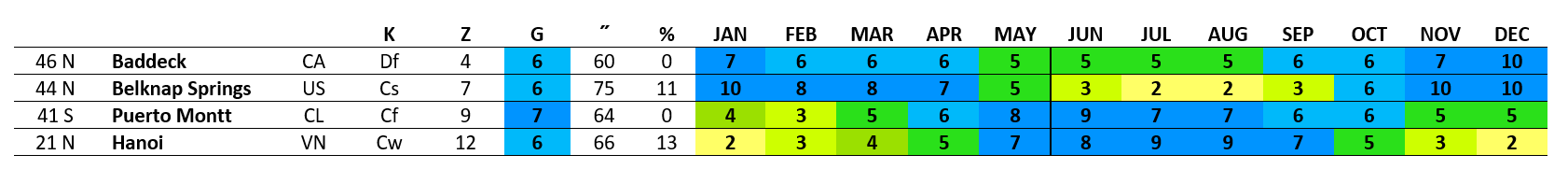
The L & L system is based on monthly temperature and precipitation averages, each of which are considered as climatic “distances” and “weights”. Hence, there are actually two very different kinds of zones reflecting the two basic ways to consider each temperature and precipitation. The “zone” used in its specific sense or as distinguished from the grade is simply a shorthand of temperature and precipitation totals as calculated over a period of time, for example, daily high and low temperatures as averaged out month by month or combined into an annual average. Unless otherwise specified, a temperature zone is based on the coldest month of the year in any given location because this represents one of those points where climates are most clearly differentiated from one another. As such, when we contrast, for example, Minneapolis in zone 3, with Nashville in zone 8, and Tampa in zone 12, we get a clear sense of the climatic “distance” between these different locations and are already beginning to speak and understand our “climate language” just that easily. If, on the other hand, we compared these same locations by their warmest month of the year on average, they would appear nearly identical: Minneapolis summer-zone 15, Nashville 16, and Tampa 17.

Of course a contrasting of climates by temperature zones is only the beginning: a climate cannot be fully identified without an understanding of its seasonal differences. Thus, whether we are talking about temperature or precipitation, when we refer to a “grade” we are referring to a zone as calculated against a period of time—which is also a number and part of the calculation—or according to its “weight” or “density”. The grade is therefore a relative number or an index of seasonality. Grades provide us with an overall impression of the climate and corresponding environment or, in other words, the “sum total” of its seasonality.

The formulations are few and simple. Their accuracy is of course dependent on the climate data, which, unfortunately, is not always consistent. Apart from that, it is really a question of understanding what the numbers are measuring and what limits these measurements have once applied to a description of the environment. The purpose of this presentation being practical as well as theoretical, we define a climate by its two most “immediate” numbers—the temperature zone and the precipitation grade. With just these two numbers and their derivatives we have already acquired half of the “language” of climate classification. The zone and grade of a single location—preferably your own to start—thus serves as a reference point to much of the remaining system.

The precipitation grade is the “parent-figure” of another figure called the aridity index, the latter which defines the seasonality of precipitation specifically. The importance of these figures especially stands out when we look at the way precipitation is currently considered in climate classification. In Koppen’s system, for example, we find entirely irregular calculations of seasonality, while in Holdridge’s system the closest thing we get to a seasonality figure is a calculation of precipitation minus estimated water loss due to evaporation, hence according to the effects of temperature primarily. This “adjustment” of precipitation totals is not in any way a substitute for a definition of seasonality, yet it is very much part of the identification of Holdridge’s ecological zones and will quickly lead to some major classification problems which we will get into shortly.

The problem regarding precipitation classification is very simple: whereas when it comes to temperature we can measure hot and cold, when it comes to precipitation we can’t measure wet and dry: we can only measure “wet” (precipitation) and the measurement of “wet”, while critical, is not always enough to get a clear or even accurate overall picture of the climate in question. The precipitation grade and derivative aridity index are designed to solve this problem, the former providing a “sum total” of “wetness”—the grade also has a kind of partial calculation of seasonality within it—and the latter a “sum total” of “dryness” given as a percentage—in short, wet and dry on the balance sheet of things.

All of the above figures are completely new to the subject, each having their assigned roles and limitations. The next major figure, however—the temperature grade or warmth index—is based on Holdridge’s biotemperature. Holdridge’s term will be regularly used in the content to follow but it is a bit narrow in that, like every other figure of climate classification, it describes not only bioclimates but also certain aspects of climate more generally, that is, independent of the ecology. Again, the most significant difference between the temperature grade and the temperature zone is that the former measures the “weight” of the seasonality of temperature, by which it is meant the sum total of “warmth” or temperatures above freezing—something which the latter can only approximate and only if we include the summer-zone. On the other hand, in climates having monthly averages at or below freezing, a “0” rather than a specific temperature is registered when we use the temperature grade. Ultimately, of course, the two figures complement one another, both contributing to our understanding of the climate in question.

The last major figure is that of the precipitation zone, again a fancy term for what is simply a shorthand figure. Apart from the snow zones, these have not yet been included although these are important and can be absolutely critical in any number of ways. For basic climate classification, however—which is our goal here—owing to the great diversity of seasonal precipitation across the globe, the precipitation grade and aridity index are so much more telltale than annual precipitation totals or the more general precipitation zone. For example, Mumbai has an average annual precipitation of 87”(precipitation zone 8 or 7’3’’) and can easily be regarded as “very wet”. In contrast, Chicago with 39”/yr (zone 4 or 3’3”) can be regarded “semi-wet”. The difference between the two, however, is that in Chicago the precipitation is distributed more or less evenly throughout the year whereas in Mumbai 95% of the precipitation is distributed in just 4 months, practically the remainder of the year being as dry as a desert. Thus, to characterize Mumbai simply as “very wet”, while not false, provides no relevant detail especially given that its climate as viewed across the year appears much more “desert-dry” than “very wet”. These seasonal differences are easily measured by the aridity index and thus help us to characterize the climate in a much more meaningful way: Mumbai the very dry forest—the “forest” (grade 5) being regarded “wet” in this system—and Chicago the woodland (grade 4), regarded “semi-wet”.

Many other figures are found in climatology and climate classification. Some of these can be adapted to the methodology of zones versus grades, if not right into their actual system. The temperature zone, for example, can be easily turned into a cold-hardiness temperature zone, hence expanding not only our “climate language” and its use as a tool of comparison even further, but also contributing to the definition of plant-cold hardiness.

the USDA plant cold hardiness zones

If you’re not into gardening you may not be familiar with this interesting little system. Current and past hardiness zone maps can be easily found on the internet, but back in the day people would have probably only seen such a map whenever they bought a packet of seeds, a small zone map of the US being found on the backside of the package. In fact it was this map and the simplicity of the system itself that in many ways inspired this project: the zone number represents a climatic “distance” making comparisons between locations a very definite thing, hence, also easy to use and remember. Moreover, having a practical purpose, it may very well be the only commonly known “climate number” for many people and certainly much more known than something like the average annual temperature of one’s own location.

The temperature zones in fact generally resemble the hardiness zones although they are calculated in a completely different way. The hardiness zones are based on the average lowest temperature of the year. There are 13 such zones, each 10˚F apart from the next; some websites add on a few more zones. The temperature zones are different because they are based on the average temperature of the coldest month of the year—a much easier figure to find, incidentally. However, unlike the hardiness zones which have a singular purpose, the calculation used to determine a temperature zone can also be used to define many other aspects of the climate in question. Besides defining some aspects of plant cold hardiness, they can also be used to define the differences between climates, seasons, and more. There are around 36 temperature zones and they are divided into groups of 4, each group representing a more general climate type such as temperate (zones 5, 6, 7, 8); subtropical (zones 9, 10, 11, 12), and so forth. As stated above, together with the precipitation grades we have a very easy-to-use language in the subject of climate classification. Here we are going to examine in practical terms how the new zones compare to the USDA hardiness zones, how each of these systems are in fact limited even when it comes to assessing plant-cold tolerance, and how the hardiness zones can be modified so as to result in yet another use of the temperature zones.

When the USDA zone map first appeared in 1960 Miami and Los Angeles both appeared in hardiness zone 10—yet Miami has a tropical climate and has, for example, coconut palm trees growing there, while LA has a Mediterranean climate and does not. One could reasonably come to the conclusion that the “success” of the coconut palm was questionable in zone 10: if the conditions were just so it will survive, if not, it won’t. It appeared almost a matter of luck at this point rather than climate—hope was offered for anyone interested in growing tropical plants in the deep south of the United States.

The adjustments in the more recent hardiness zone maps only added to the confusion with regard to this particular question. The original map, limited to the 48 contiguous states of the US, only went up to zone 10 which, in turn, might explain why Miami and LA were bunched together, that is, if we were to interpret zone 10 as “10 and higher”. How do these cities compare in the updated maps which go up to zone 13?

In the 2012 USDA map, Miami belongs to zone 10b and 11a. The new zone (11a) might have been the improvement we were looking for, that is, until we come to the realization that LA was also placed in 10b and 11a. Perhaps we should conclude from this that LA is mostly in 10b and Miami mostly in 11a. This would suggest that the main territory of the coconut palm tree begins in 11a—most of Miami by this way of thinking, but is virtually unknown in 10b. This might explain its absence in Los Angeles.

Unfortunately, the system of hardiness zones does not actually allow for this possible explanation. Take the case of Tampa in central Florida near the Gulf of Mexico. The more northerly part of the city is listed as 9b, while the southerly part of the city, especially near Tampa Bay itself, is listed as 10a. Although fully a zone below Miami the coconut palm tree can still be found, although it may be periodically damaged or even killed by any severe or prolonged frost. Are we to assume at this point that 9b represents the “absolute lowest limit” for the coconut palm? The system of hardiness zones would indeed have us believe that and, indeed, the USDA declares the coconut palm tree to be hardy to zone 10a and higher, and possible in very small microclimates in 9b.

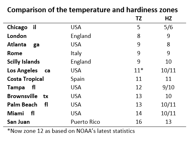
With a slightly modified version of the system applied to more and more countries its validity becomes even more suspect. Places like England’s Scilly Islands and some southwestern coastal strips in Ireland, for example, are said to be in zone 10—just like Tampa close to the bay—except of course the coconut palm tree is nowhere to be found. Other locations too, like Rome, where the hardier date palm can be (or has been) grown ornamentally, is listed as 9b just like north Tampa. Even Dublin or London—depending on the source or perhaps the reading station—are sometimes determined to be in 9a: are these locations just barely beyond the reach of enjoying some tropical imagery?

There are, however, warmer locations in Europe: Lisbon is found in zone 11, and, unlike Miami, there is no mention of 10b. Could Lisbon be more tropical than Miami in terms of plant hardiness? There is also Spain’s Costa Tropical centered around Almuñecar—also in zone 11—where some typically tropical plants are indeed cultivated: guava, mangoes, and, at least until recently, sugarcane—yet again, no coconut palm trees.

To be clear, it is possible for a coconut tree to prosper for a period in a near-tropical climate such as we find in Tampa in central Florida. But there are or have been a handful of reported cases of coconut palm trees growing in southern California where the climate is considered fully subtropical. These would appear to be on the very limit of what is possible. The Newport Beach palm (south of LA) planted in the mid-eighties survived until 2014; another said to be growing in La Quinta and another in San Diego, and who knows where else. However, the Newport palm was very stunted (unlike those found in Tampa) and could not produce a single coconut. It was also planted against a south-facing wall to amplify the temperature a little bit during winter. Ultimately, it had less than half the normal life span of the species.

The case of the coconut palm tree demonstrates some of the problems with the USDA hardiness zones. Is this system really addressing what we need to understand regarding a plant’s cold hardiness? Or does it lead to wishful thinking amongst people who like growing exotic plants? Also, where do the tropical climates begin in all this? How do they relate to the zones? It seems as if Mediterranean LA and tropical Miami should be on opposite sides of some climate border. Meanwhile, looking further, San Juan Puerto Rico is fully 2 hardiness zones higher than Miami. Is Miami really more like Los Angeles in terms of plant cold hardiness?

And what about those tropical plants grown along the Costa Tropical? It turns out that sugarcane, for example, although widely grown in tropical climates can also be cultivated in hotter subtropical climates as well.

It seems like wishful thinking or the desire to grow plants outside their prescribed zone is kind of built into the system of hardiness zones by way of the contradictory “conclusions” that can be drawn from it. If, for example, the coconut palm cannot grow in Lisbon which is in the same zone as Miami, then, following this logic we would be led to belief that not low winter-months temperatures but some other condition or combination of conditions is the reason why this must be so: the soil type or its temperature, sunshine hours, humidity, and precipitation, etc. Yet it is not hard to see that we can control certain things like the soil type, water, etc., so what is the real difference between these two cities? What is the purpose of saying the coconut palm tree is hardy to zone 9b, 10a, 10b, or even 11 if it cannot grow in most of zone 11?

The problems in the system of hardiness zones have led some to the conclusion that the zones are valid—but only in the eastern US—and that other regions require other systems or modifications to the original USDA hardiness zones.

The temperature zones provide a clearer picture and great starting point wherever we go. Further, they are fairly compatible with the existing system of hardiness zones, especially once we exclude what are usually considered to be tropical climates:

The results obtained using the temperature zones are altogether clearer, and can therefore act as a general measurement of cold hardiness at least as much as the cold hardiness zones themselves, both being subject to limitations in their application. There is indeed a reason, even a number of reasons, why the coconut palm is “hardy to zones 9b and higher” and yet is still quite absent even in zone 11. For the most part in any case, the coconut palm tree flourishes in temperature zones 13 and higher, whereas in zone 12 all the right conditions have to be present so that it can reach maturity and reproduce. In the case of Tampa it can sometimes do this before any freezing temperatures or prolonged cold are serious enough to damage or kill the specimen altogether. Using temperature zones we can already see that Los Angeles is differentiated from places like Palm Beach (so named for its coconut palm trees by the way) and even more from Miami; that places like Dublin and London, are not a zone or so away from Miami, but rather 5 or 6 zones away. Furthermore, we see that Miami is well within the tropical climate zone—which begins at 13 and is closer to San Juan in this respect—not Los Angeles as the hardiness zones would make it appear.

Additionally, since average monthly temperatures are probably the easiest statistic to find, anyone can determine their own temperature zone or at least that of the nearest reading station. Simply add the average high and low of the coldest month of the year wherever it may occur–usually January in the northern hemisphere and July in the southern hemisphere—and divide the result by 10. When only the daily mean is provided, this figure is doubled before dividing by 10. To be noted in this system, a result such as 9.49 for example, is not rounded to 9.5 (= zone 10) but simply left at 9.4 (= zone 9) as this is more in line with the issue of plant-cold hardiness and the differentiation of climates according to the coldest average monthly temperature of the year. Also note that for some agencies the daily mean is not necessarily the average of the mean daily maximum + mean daily minimum, the latter which we use whenever possible.
The use of the temperature zones does not put an end to the question of plant cold hardiness. There often are some significant differences between, for example, temperature zone 9 in the eastern US (for example, Atlanta) and zone 9 in other locations where, for example, winter’s low temperatures may be moderated by proximity to the ocean or the zone is shielded somewhat from the polar winter by mountains. Additionally, there are other considerations when determining the hardiness of a species according to temperature, for example cool hardiness or tolerance which is not only applicable to winter temperatures but also summer temperatures. One of the advantages to the system of temperature zones is that they may adapted to define cold hardiness specifically, as well as cool hardiness, heat tolerance and so forth, the same system of numbers being used throughout.

If one’s sole purpose is to grow a plant at or even beyond the limit of its native environment, then the question of how cold it can get in a specific location is very important. This question, however, can be assessed in relationship to the temperature zones. In this way we have the added benefit of seeing the absolute difference between the temperature zone and the average coldest temperature of the year (as part of the determination of a zone number). At present, this will require a little research for any enthusiasts out there—either several years of monitoring the temperatures or researching local weather records in their own location for the duration of the cold months.

Chicago, for example, is in zone 5 (both its temperature zone and its USDA hardiness zone). Using the new system we would discover that its coldest day of the year is equivalent to zone ‒1. This is only based on temperatures from the last winter—12/23 through 2/24)—but it gives us a rough idea of how a hardiness zone contrasts with the temperature zone. In any case, it is a much more graphic and sure way to assess any significant differences between temperature zone 10 in say northern Florida, and temperature zone 10 in California, Texas, southern France, etc., or in specific locations within these regions.

Transition zone in Florida

The temperature zones shown thus far have been rounded off which is good enough for most practical purposes and general discussions. Like the hardiness zones they can be further distinguished by dividing them in two, “a” representing the cooler half and “b” the warmer half. The new calculation allows for even finer distinctions as you will see below.

Florida is a good place to observe the transition from the subtropical to tropical climate since the state is very flat and, of course, part of the US mainland, most of which is regularly subject to freezing temperatures in winter. The long-term survival of the coconut palm tree generally extends from Punta Gorda (Charlotte County) on the western coast of the state and Stuart (St. Lucie County) on the Atlantic coast—along the coasts somewhat further north still. These locations correspond with zone 13 in the new system—the first of the tropical zones.

A close-up look at the zones in any region is of course limited to the number of reading stations, the number of years of collected data and time frame (30 years is the standard), and the accuracy of available sources. For the present purposes, we can only assume that a typically tropical plant grown in 12.4 will do better than one in 12.3 which in turn will do better than one in 12.2 and so on. Certainly many other factors contribute to the success of a plant in a borderline situation where winter temperatures are already causing enough stress on it: soil and nutrition, sunlight hours, moisture, the age of the plant, etc., in short, the overall health of the plant to begin with. It therefore happens that some plants in borderline situations survive a cold spell while others of the same species and sometimes even in the same proximity do not.

Some cities shown below have more than one zone number. This is because multiple internet sources were consulted; the reader may find still others in the locations of interest.

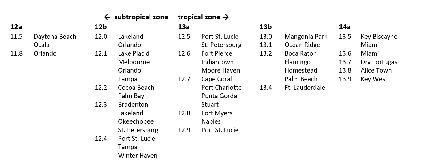
As could be gleaned from the internet—and not necessarily on the authority of local experts and knowledgeable plant enthusiasts—the success of the coconut palm and other tropical plants varies considerably in 12b: St. Petersburg (12.3, but also 12.5 which is tropical) has tropical plants in many parts of the city. The coconut trees are planted from seeds and can bear many coconuts if they can reach maturity and survive the winter. Likewise Orlando (11.8, 12.0, 12.1) except that they are harder to find and do not always reach their full stature. All of 12b in Florida is subject to periodic freezes and cold spells that could seriously damage any frost-sensitive species, more so in Orlando than St. Petersburg judging both from the numbers and the descriptions regarding the quantity and quality of tropical plants in the two locations.

It goes without saying that in Florida, minus the Florida Keys which have no recorded frosts, these cold events occasionally penetrate zone 13 and beyond, but with less and less frequency and intensity and consequently with less and less devastating effects. Conversely, 12b locations can have many years of zone 13-like winters. The frequency, duration and amount (degree) of cold are obvious major considerations in assessing cold hardiness—all of which, as a general rule, are taken into account in a system defined by averages—the system of temperature zones.

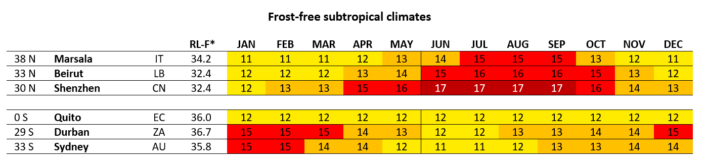
Unlike Florida, where even the tropical climate zone is occasionally penetrated by freezing temperatures, there are also subtropical localities and regions (almost all in zones 11 and 12) that experience very little or no frost at all. This includes southeastern China, part of which is actually located in the tropical latitudes; various highlands within the tropical latitudes; various locations within and near the Mediterranean climate regions, and so forth. Even in these frost-free environments, however, the rather cool winters make growing many tropical species difficult or very unlikely. Again, this is not necessarily because they cannot withstand occasional freezing temperatures—although some tropical species can’t tolerate any frost—but rather because they cannot withstand a period of prolonged relatively cool temperatures. Similarly, in the case of some tropical-climate highlands, the very short or absent hot season indicative of a mild-summer climate year-round also prevents the successful growing of many tropical species. Later on, using biotemperature, we will learn how the differences in year-round “warmth” add up to what is effectively a more subtropical or sometimes even a more temperate climate, that is, in spite of the fact that a zone 13 or tropical climate is otherwise indicated.

Again, in spite of the numerous advantages of the temperature zones, they remain limited by what they measure—the average temperature (mean daily in the US) of the coldest month of the year. This is not the same as the average temperature of the coldest day of the year or, in the case of the cold hardiness zones, the average coldest temperature of the year.

Koppen’s climate classification

This is basically the oldest system of world-wide climate classification, although parts of the subject date back at least to the Ancient Greeks from where we derive such terms as climate, arctic, antarctic, and tropic.

Koppen’s system identifies 30 different climates—each with 3 letters—according to the level and seasonality of temperature and precipitation. The consideration and calculation of seasonality is a big plus historically. On the downside, the organization of the system is on the chaotic side. This begins in the foundation itself with the principal categories: tropical, dry, subtropical, etc., and continues within these main groups, each following its own standards and formulations which of course is reflected in its system of letters too. So while the 3-letter system certainly looks appealing, the letters neither represent uniform “weights” and “distances”, nor are enough to clearly identify the main differences between climates. Hence, in spite of numerous revisions of the system, closely related climates are still often separated from each other, and vice versa, very different climates are often joined together.

Unlike the hardiness zones where the main problem mostly involves tropical locations, the Koppen demarcation of the tropical climate is basically in agreement with the system presented here. This time, however, most of the remaining system is not. Whereas his tropical climate spans 4 temperature zones (like ours), his subtropical climates span 7 zones, his humid continental 8 zones, and subarctic climates 17 zones. Whatever the logic in this organization of climates, the end results are clearly unsatisfactory.

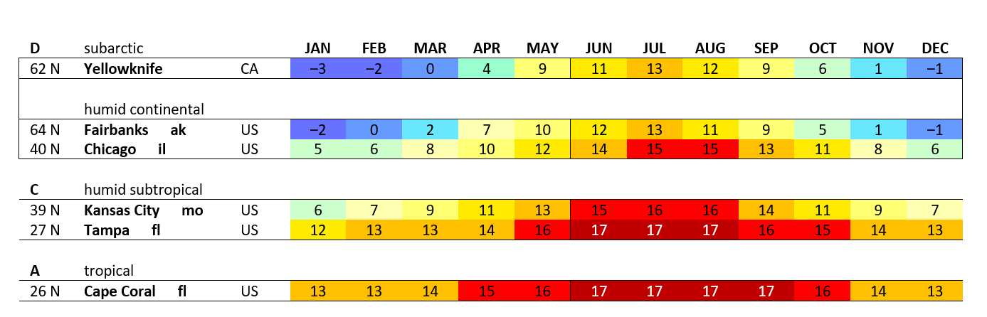
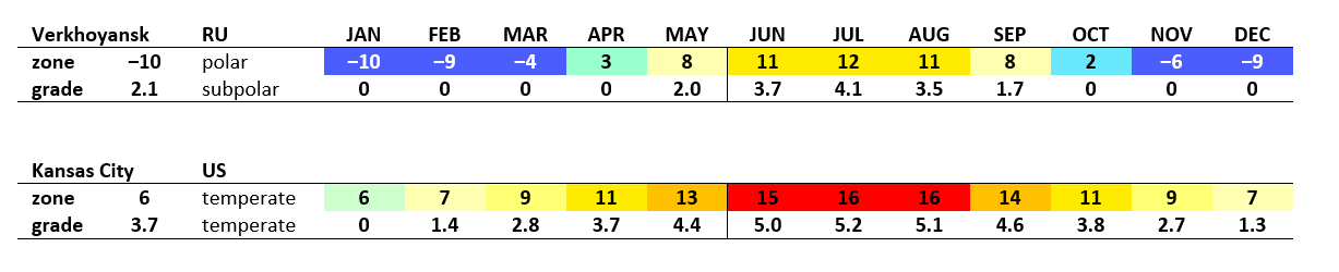
These great climatic distances cannot be justified. Although Kansas City is found in the same category as Tampa, it is clearly much more like Chicago in the cool temperate zone. Chicago and KC generally experience the same weather phenomena, share the same hardiness zone (5 or 6), a similar plant and animal life, agricultural products, etc. The situation in Florida is obviously altogether different: a dozen native species of palm trees, frost-sensitive agricultural products including citrus fruits and sugarcane to name the most common, gardening seasons often before and after the very hot summers, crocodiles inhabiting its tropical south, alligators the subtropical regions as well, a tropical storm and hurricane season, and so on.

The same kind of misclassification also occurs between Chicago and Fairbanks, except that the “distance” between the two is even wider. That there appears to be no significant climate border between humid continental Fairbanks and subarctic Yellowknife is already questionable, although in every system a line has to be drawn at some point. By zones, both locations are considered polar; by grades, subpolar. In the case of humid continental Chicago and Fairbanks, however, we see two very different climates, yet the only difference identified by the Koppen system is that Fairbanks has a warm summer (Dfb) and Chicago a hot summer (Dfa). Obviously the differences in climate between these two locations is much more significant: winter (as zone 6 and lower) is 6 months long in Fairbanks and 3 months long in Chicago. Summer, in the sense of the tropical range of temperatures, is 1 month long in Fairbanks and 4 months long in Chicago. Fairbanks is in hardiness zone 1 or 2, has a growing season of 116 days, and record lows in summer below freezing; it is located in the boreal forest region. Chicago is in hardiness zone 5 or 6, has a growing season of 187 days, and is located within a temperate deciduous forest region. It should also be pointed out that Fairbanks is color-coded on Koppen-based climate maps to appear as a subarctic climate; this will turn out to be a regular occurrence when the Koppen formulations create glaring contradictions once being mapped out.

Both the foundation and internal divisions of the Koppen climate classes lead to numerous examples of misclassification of this sort. Without a standard of measurement applicable to all locations an accurate and comprehensive view or the earth’s climates is not possible.

Precipitation classifications

The Koppen precipitation classifications and designations are even more contradictory.

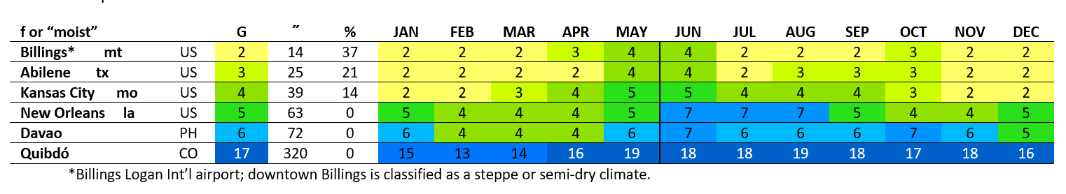
Notice the expression “classifications and designations”: Koppen put the desert and semi-dry climates which otherwise fall in the range of temperatures in classes A, C, and D, into a class of their own—group B. Thus, in groups A, C, and D, the precipitation type appears as a designation—f, m, w and s. Thus, every location that does not qualify as desert or steppe (group B), or tundra or ice cap (group E), is either humid (moist) or at least “not dry,” that is, not dry enough to fall into his semi-dry category. Only the f-climate is actually called that, however—the f literally translating German feucht = moist, meaning “moist all year”. The first thing to do then is see just how feucht these climates really are:

It turns out that that not all of the dry climates have actually made it into Koppen’s B group. Thus, the f or “moist-all-year” designation is also apparently interpreted as “no distinctly dry or wet season”. Thus, a very wide range of grades and aridity percentages are represented by “f”, in short, anything from a brushland to a very rainy rainforest, or, by definition, any climate where the precipitation pattern is basically uniform throughout the year which, technically speaking, can include the polar and most hot deserts as well.

Verkhoyansk Russia—an “f” climate—does actually qualify as a desert if we use the figures provided by the National Oceanic and Atmospheric Administration (NOAA) which counts only 35 precipitation days/yr—52 days would be required to place the town in the brushland grade. Statistics from Russia show 184 days with rain and/or snow which places Verkhoyansk in the brushland range. The Russian figures are only possible if the threshold defining a rain and/or snow day is very low—0.01 mm possibly? Any day with any amount of rain and/or snow? This could not be determined.

Even within a specific climate category the f precipitation type can be regarded as way too general: In the chart below, for example, Abilene and New Orleans are not just in the same precipitation group, they are also in the exact same classification—Cfa—that is, in spite of their differences in annual precipitation (38”), their aridity index (21%), number of dry months (10), and by grades (2). From the standpoint of the grade system is doesn’t make sense that grade 3 or semi-dry Abilene—additionally, a place where only 2 months of the year fall in the wet grades—should be grouped with the humid subtropical climates in the first place.

The remaining seasonal designations are not quite this wide but will also result in major classification problems, especially when the Koppen categories are thought of as bioclimates.

In any case, the grade system eliminates the progression: desert (dry)—semi-dry—wide range of moist or seasonally moist climates, in favor of: desert (very dry)—dry—semidry—semi-wet, etc. Nor will there be any need to have a separate category for the drier climates (Koppen’s desert and semi-dry climates). These are about equivalent to grades 1 and 2—very dry and dry, respectively, and will be found in every temperature group.

Southern California and the “aridity line”

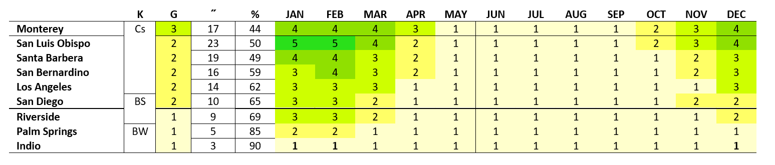
The separation of the drier climates from their temperature ranges can also sometimes result in an unnecessary distinction between a semi-dry climate and a virtually identical dry climate still classified in one of the temperature groups, that is, for not having quite met the qualifications of the semi-dry category. In such instances the semi-dry climate appears like a kind of buffer zone between the “nearly semi-dry” climate and the desert. One has to wonder then, what meaningful boundary can be found between, say, semi-dry Riverside or San Diego and Mediterranean Los Angeles? If perhaps one or both of these locations qualified as deserts such as we find in nearby Palm Springs, then we could certainly say a more definitive boundary has been crossed.

The grade system and aridity percentage take out the guess work and leave only one border left standing, the border between grade 1 and grade 2, that is, between the desert or very dry climates and the dry climates. This border is very significant indeed. In fact, it is going to have the same significance for climate classification with respect to precipitation as the “frost line” between the tropical and subtropical climates has with respect to temperature. On the tropical side of the border at 12.5 (zone 13) temperatures are warm and/or hot year-round and frost is absent or very nearly so at its fringes. The border of the desert climate begins at an aridity index of 66.6%. The desert is a region of little or no precipitation and consequently a region where the vegetation is scarce or completely absent, barring of course some other source of water. Thus, the tropical climate and desert, limited at 12.5 and 66.6% respectively, become the “measuring stick” of two fundamental aspects of climate classification, temperature and precipitation.

The borders determined by the thresholds of climate classification are “fluid”—even more so when the two zones meet up with each other on a more or less uniform terrain. At the frost and aridity line, for example, first in the sense that occasional frosts and (relatively) excessive rains sometimes cross into the tropical and desert regions, respectively, and second in that both sides of any border will clearly have more in common with each other than with the opposite ends of their own zones. This is not a problem for climate classification, that is, unless the basis of a particular threshold is not clearly defined and/or the two climatic regions forming the border have very wide and irregular ranges—which are exactly the kinds of problems we encounter in Koppen’s system. The bottom line here is that, for the purposes of climate classification, the frost and aridity line are absolutely indispensable.

As for southern California, as measured by the grade system, we see that Riverside has in fact crossed into the desert category, while San Diego has joined Los Angeles in the Mediterranean climate group, its driest type. One can still discern a Mediterranean pattern in Riverside, but the increasing aridity is already leveling out and erasing any seasonal differences. If a desert is large enough and dry enough, every last trace of the seasonality found on its fringes could eventually disappear altogether. In Indio we still see trace amounts of the Mediterranean seasonality, the 3 wettest months being shown in bold print because no change of grade was involved.

Floristic and geographic regions

Although Koppen’s system is often described as “vegetation-based”, most of the categories are too wide and irregular to have any real meaning. When it comes down to it there are only 4 “official” ecosystems identified in Koppen’s system—the steppe and the tundra, the desert and ice cap (polar desert)—plus the tropical moist forest (Af), usually equated with an evergreen rainforest. The few other equations of the letter-system with particular ecosystems are quite indefinite. All in all it is very hard to see how such a system can be considered useful to the determination of vegetation zones with respect to climate change and climate change scenarios such as is commonly claimed.

The Koppen system is sometimes referred to as a “geographer’s system”: categories A through E—tropical through ice cap—plus the calculations of seasonality are indeed general reflections of the earth’s geography, its corresponding atmospheric circulation, and so forth. Again, however, the 3-letter system and their formulations greatly limit what is otherwise the most interesting aspect of his system.

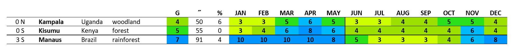
There is general agreement between Koppen’s tropical rainforests (Af) and those defined by grades and the aridity index—for one thing, some locations are just “too wet” to leave any room for a dispute. There are some climates, however, that do not fall in the rainforest grade but are considered rainforests in the Koppen system, for example, Kampala and Kisumu, compared below with Manaus:

Many tropical climates that qualify as rainforests in the grade system are found in Koppen’s so-called monsoon category. San Juan is at least one example of a climate that is regularly color-coded as a rainforest climate on Koppen-based maps in spite of the fact that it is found in the monsoon category.

The rainforest climates in groups C and D, even those with the f-designation, are not identified as such. As we have seen earlier the f-designation can mean almost anything outside of group A.

Koppen’s monsoon climate is only identified in group A, tropical, even though the same phenomenon occurs in all of the temperature classes: subtropical, temperate, etc. However, Koppen does not actually use the term to describe climates where the monsoon—generally characterized by its seasonally reversing winds and its causes—is well developed, but mainly to describe a transitional zone between the tropical rainforest which is basically wet all year and the tropical savanna climate, which may have a rainy season but is dry much of the year. Hence, it is intended to describe a seasonally dry rainforest or jungle. In any case, it is not a useful term at this level of climate classification: in terms of monthly and yearly averages—the starting point in climate classification—the many precipitation patterns in India at least generally resemble what we find in other regions of the world whether the monsoon is fully defined, partially defined (Mexico and the American southwest), “split” (Africa), notably supplemented, or not defined at all.

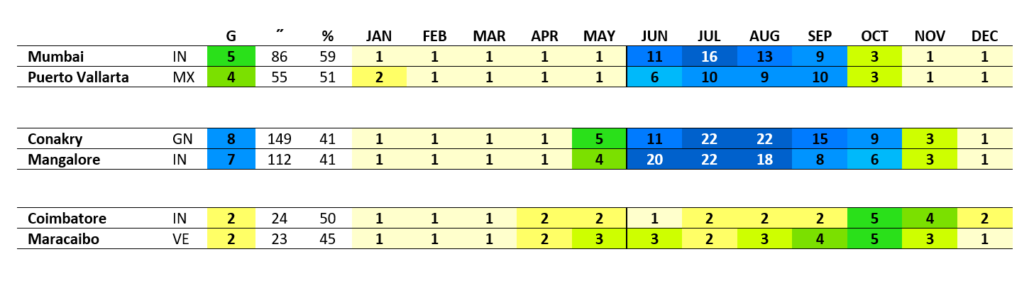
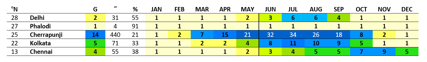
Mumbai, Mangalore, and Coimbatore shown above and all of the following locations in India are affected by the monsoon, yet only Mangalore is part of Koppen’s monsoon category. The wetter summer in Phalodi located in the Thar desert does not cause a change of grade.

Although Koppen’s monsoon category does not refer to any ecosystem, it is broadly associated with the tropical seasonal or partially deciduous rainforest—the jungle—which is found wherever there is a significant dry season. Its association with a relatively wet environment—for example, as found in Koppen’s monsoon category—is contrary to its original sense: Sanskrit jangala meaning “arid”. In Hindi, however, jangal acquired more the sense of “unsuitable for cultivation”, referring, so it seems,  to any number of environments from the desert and scrubland to the dense thickets of the seasonal tropical forest.

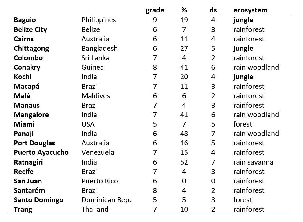
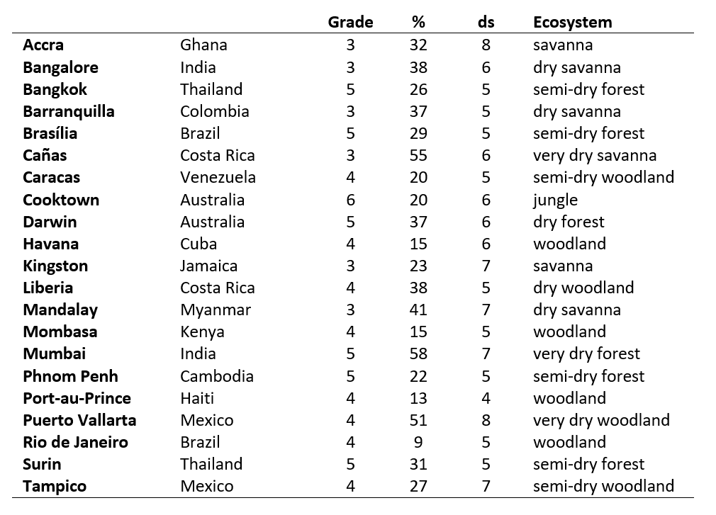
The following cities are typical of Koppen’s monsoon category, although some can be found in other categories too depending on the source, the statistics being used, the version of the Koppen system being followed, etc. Here they are re-evaluated using the grade system. In spite of the relatively small geographic territory occupied by Koppen’s monsoon climates, the aridity index in the cities shown below varies from 0 to 52% and the number of months per year that fall in the dry grades (ds, that is, the whole dry season) vary from 0 to 7—the rest of the year constituting the wet season. The newly defined “ecosystem” or bioclimate is based on the grade and the aridity index. The exact length of the dry season by monthly averages is a bonus figure that comes with the grade system and gives an indication as to how the aridity is spread out; however, it is not actually part of the determination.

As can be seen in the examples below, only a few of these fit the more or less common conception of the jungle as defined above; the 3 rain woodlands shown have desert-dry seasons lasting 5 to 6 months, which of course will impact the ecosystem in a very fundamental way. Miami’s dry season is also quite long, but consists of 5 semi-dry months (as opposed to desert-dry and/or dry months) and so is very different in terms of its ecological impact. This is reflected in its low aridity percentage—had these been 5 desert-dry months, for example, Miami’s aridity percentage would jump from 7% to somewhere between 28% and 42% and its forest climate would turn into a semi-dry forest or dry forest climate, respectively.

Koppen’s As and Aw climates are often called the tropical savanna or tropical wet and dry climates. These are the last and the driest of the specifically tropical categories, everything drier falling in category B. The s designates a drier “summer” pattern (high sun) and the w refers to the much more common drier “winter” pattern (low sun). The distinction serves little purpose in the tropics and can be very hard if not impossible to determine along and near the equator where “high sun” actually occurs in March and September. Either way, both are considered savanna climates.

Once again, although only indicated in the tropical group, the savanna can also be found in subtropical, temperate, subpolar, and polar zones as well. Following is a list of cities listed under the category As or Aw and their re-evaluation using the system of grades. A close-up look at the climates of the Yucatan peninsula follows the main list.

The Yucatan Peninsula

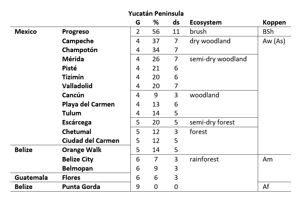
The flat terrain of the Yucatan peninsula is a good place to observe the gradual transformation of the natural environment. Its biomes consist of deciduous forests, especially in the northwest—excluding the dry climate around Progreso—and semi-deciduous and evergreen forests everywhere else. Minus the Progreso region, and excluding the states of Tabasco and Veracruz, parts of which could be considered part or the peninsula but are not included here, the whole of the northern, Mexican portion of the peninsula has a savanna climate according to the Koppen formulations. The problem here is that, taken as a whole, the region is not associated with the savanna, but with the forest (admittedly these are general terms) and, in any case, the several types of forests are not distinguished in any way by the Koppen system. Significant contradictions between the classification and the actual biome (or even the actual climate) have led to multiple revisions of the system over the years, beginning with Koppen himself. In the case of the tropical climates, however, it has mainly led to some fairly recent interpretations that do not match the Koppen formulations or its revisions: San Juan Puerto Rico, for example, although numerically part of the monsoon category, is typically color-coded on the maps so as to appear a part of the rainforest category. Similarly, the wetter or “greener” biomes within the “mathematical savanna” of the Yucatan are sometimes included with the wetter monsoon climate.

The humidity grades together with the derivative aridity percentage delineate 7 bioclimates in the Yucatan as opposed to 4 according to the Koppen standards. The new bioclimates certainly better reflect the gradual transformation of the natural environment. But do they reflect the biomes of the Yucatan loosely or in a big way? That’s a little harder to determine since the descriptions and maps of the biomes (at least as researched on the internet) are generally vague and often contradictory. To be sure there are some clear-cut cases not appearing to be disputed anywhere as far as we know: the rainforest climate of Punta Gorda Belize, for example, matches its rainforest biome and likewise the brushland around Progreso matches its bioclimate. But what about the dry woodland, semi-dry woodland, and other bioclimates?

If we compare the dry woodland climate of Campeche and Champotón with the dry woodland climate of Liberia Costa Rica (shown above), the latter which matches the well-known deciduous woodland of the nearby Guanacaste National Park, we would certainly think that the dry woodland climate at least roughly corresponds with a deciduous biome. Logically, it would follow that the semi-dry woodland climate correspond roughly with a semi-deciduous biome as the aridity percentage is lower and the dry season is up to a month shorter or at any rate less intense; the woodland and forest bioclimates with a more or less evergreen forest, because the aridity percentage is even lower and the dry season even shorter as a whole, and so forth.

Whatever the case may be, the bioclimate can only provide us with a general picture, since it is based on general information and does not take into consideration any other factors which can result in a “mismatch” between the climate and the biome.

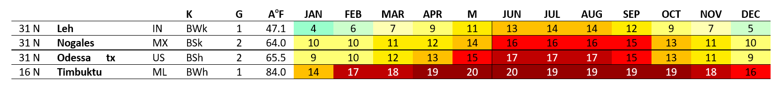
Koppen’s semi-dry or steppe (grassland) category is about equal to our grade 2, dry. It is divided at an average annual temperature of 64.4^oF (18^oC) into cold and hot so that the cold temperate steppe and the hot tropical and subtropical steppe (or savanna, but not Koppen’s tropical savanna climate, Aw and As) grade into the cold and hot desert, respectively. This division leads directly to misclassification and some misleading descriptions of climate in various locations.

In terms of temperatures, the otherwise subtropical Nogales is simply “cold” and classified with Leh India which dips into the subpolar range of temperatures, while nearly identical Odessa is “hot” and is classified with tropical Timbuktu.

There is not actually agreement concerning the nature of the ecosystems found in the equivalent of our grade 2. Koppen’s system is more or less in line with an old yet persisting idea whereby the temperate and tropical grasslands constitute the two main grassland regions on the planet. Thus, in Koppen’s system, the desert is followed by the grassland is followed by the moist or at least moister ecosystems. In Holdridge’s system of life zones (1947), however, the scrubland is found between both the temperate and tropical grassland and the desert; Whittaker (1975), meanwhile, a temperate grassland and a tropical scrubland, each merging into the cold and hot desert, and so forth.

Biome classification and maps are not necessarily consistent either. In some maps the Australian desert is surrounded by grasslands on both its tropical and subtropical sides, in other maps and descriptions, however, a scrubland is indicated on both sides. Similarly, the Sahara by the Mediterranean scrublands, woodlands, and forests (while the natural grasslands which can indeed be found are not even mentioned); on the tropical side, the Sahelian grasslands, scrub, savannas, and woodlands…It goes without saying that some of the grasslands we see today are the end result of the erosion that followed the unchecked clearing of the land for whatever reason such as was already noted on a wide scale in Ancient Italy, Easter Island in the 17^th century, the panhandle region in Oklahoma in the 1930s, etc., etc.

So is it a brushland consisting mostly of scrubland or of grassland? In the system of life and living zones the question, although interesting enough, is not answered nor needs to be. For this reason grade 2 is called the brush or brushland: this may be about as close as we can get to a terminology in English that can be used generically, that is, if the grasses and other herbaceous plants are thought of as a “soft brush”. Our definition of the savanna—the semi-dry grade—is similar in principle, typically representing anything from a relatively taller grassland to a relatively open woodland. In any case, grade 2 may consist predominantly of either scrubland or grassland or is a mixture of both ecosystems, for example, a scrubland with a grassy understory, or a “mosaic” landscape, where one form readily gives way to the other in the same vicinity or region without any apparent change in climate. Thus, while grasslands often do constitute their own biome, they do not seem to possess their own bioclimate. In fact, although prevalent in the dry grades (except the desert), grasslands can be found in the wet grades as well: the American prairie (what’s left of it) and Eurasian steppe, for example (grades 2, 3, and 4); the Brazilian caatinga and cerrado (2, 3, 4, and 5, including seasonally flooded grasslands), etc. If we include bamboo—a member of the grass family (Poaceae) and its only member prone to forestation—or oceanic regions where the summer months are very cool, as well as various coastal regions, grades 4, 5, and 6 if not higher.

The precipitation patterns of the subtropical and continental climates are similar to those found in the tropical climates, yet there is no equation of any of these with any actual ecosystem. Thus, while Af represents the tropical rainforests, Cf and Df define anything from a rainforest to a brushland. Again, there are locations with rainforest climates in Cf and Df—as a matter of fact, also in Cs and Cw—but simply no way to differentiate these from any other ecosystems in the same category. Patterns resembling Koppen’s monsoon climate, Am, are also found, and yet there is no Cm or Dm climate category. Finally, Cw and Dw, Cs and Ds, do not represent cooler and colder versions of the tropical savanna climates.

Koppen’s Cs category quite closely represents the Mediterranean climate with its unmistakable dry summer pattern and corresponding drought-resistant vegetation. These unique characteristics are very important to climate classification because they serve as a starting point to the precipitation categories of the temperate latitude climates, or, more generally, the consideration of climate according to the large-scale circulation of the earth’s atmosphere, in particular, the formation of the subtropical high-pressure zone and the subpolar low-pressure zone. The former leads to the formation of the hot deserts and is the cause of the dry summer pattern characterizing the Mediterranean climates as well as the drier—but not dry—summer pattern of the oceanic climates.

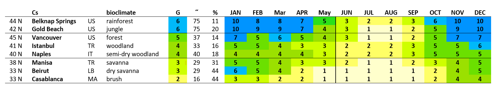
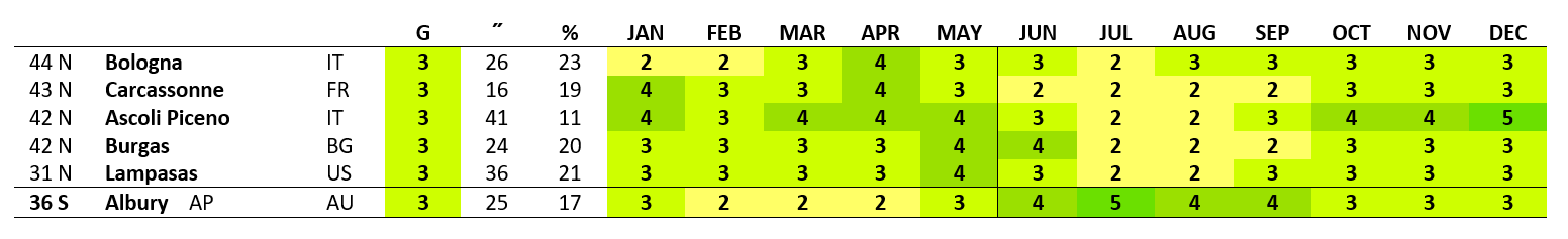
The ecoregion, although not specified by Koppen’s system, is commonly called “Mediterranean forests, woodlands, and scrub”. It is shown below in terms of the precipitation grades and aridity index. These can be subdivided: dry Mediterranean (grades 2, 3) and wet Mediterranean (4, 5), both which form the “classic” model when the location is subtropical or very nearly so; rainy Mediterranean (6+), which may also be distinguished by a cool summer (11, 12); and cold Mediterranean highlands (for example, Coeur d’Alene, Idaho) dipping into the cool temperate and subpolar zones (Ds).

The Mediterranean climate is identified by its grade 1 or 2 summer; if both the annual and summer grade are equal (for example, 2 ~ 2), the summer grade still has to be lower (that is, when not rounded off, for example, 1.87 ~ 1.25), written 2 ~ 2‒ or simply 2‒. The pattern 2 ~ 2+ or simply 2+is found in the central climates. The subtropical or Mediterranean side of the desert and the tropical or “Sahelian” side of the desert are usually differentiated in the same way: 1 ~ 1‒ and 1 ~ 1+, respectively.

In the following example, although Portsmouth England and Toulouse France look very similar in terms of precipitation, the former has a dry summer when averaged out (1.97 = grade 2), the latter, a semi-dry summer (2.18 = grade 3). Portsmouth, located on England’s southern coast, has a Mediterranean microclimate, while Toulouse has an oceanic climate even though it is very close to the Mediterranean climate region of southern Europe.

A number of Koppen’s (drier) humid subtropical climates (Cfa) actually fall into the Mediterranean category using the grade system as well, for example, Bologna which has only one month in the wet grades, or Carcassonne where the summer never even reaches the level of grade 3.

All of these determinations can change once a standard measurement of the precipitation day is adopted, for example, 0.01” (US) or 0.2mm (= 0.0078”; Canada) which are quite compatible and very suitable to basic climate classification. The standard 0.1mm (= 0.0039”) regularly employed in some countries is a little too low and the very commonly found standard 1mm (= 0.039”) is a little too high, particularly so when comparing climates that follow these standards with each other, the former which can give results that appear significantly wetter than they are (by grade and not rounded off—and aridity index) as more precipitation are being counted, and the latter drier by comparison.

The dry summer pattern defined above allows us to separate the Mediterranean climate from other temperate latitude climates as these can often be hard to distinguish from one another especially in the zones of transition. The Mediterranean climates are almost always separated from the tropical climates by the desert, whereas the central and eastern climates are directly linked to the tropics by their wetter summer. On the poleward end, the Mediterranean climates (not counting highlands) are limited by the oceanic climates whereas the oceanic, central and eastern climates are typically limited by the tundra.

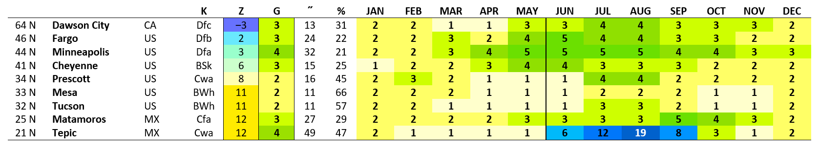
The central climates should approximate Koppen’s seasonal wetter summer climates designated by “w”, but this is often not the case. As can be seen below, many of these actually have the “f” designation in spite of their long dry season and the fact that the majority of these climates are located in the mid- through far northwest of North America. As we get close to and cross into the tropical latitudes, the wetter summer pattern may be found on either the eastern or western side of the continent, yet they still remain “central”, that is, with respect to the equatorial climate type and the tropical side of the desert—it’s a relative term—well, they all are. Like the Mediterranean climates these can be divided into dry and wet versions.

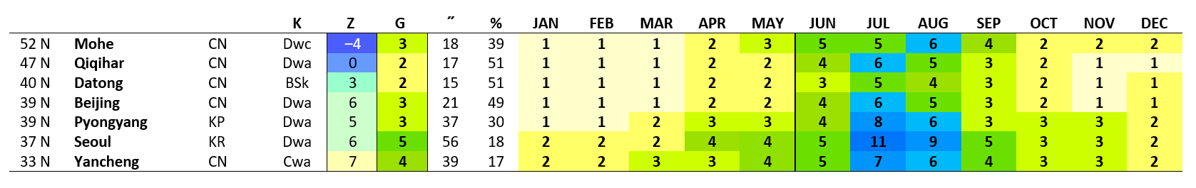
The same pattern is especially common to northeastern Asia.

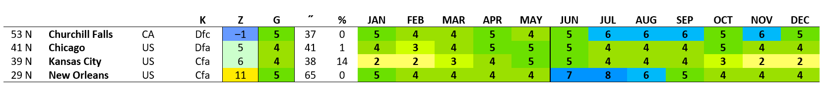
The eastern climates are simply defined by the wet grades (4+) with an aridity index at or below 16.6%. Some of these have a drier or slightly drier summer generally owing to their proximity to either the low-pressure oceanic climates or the subtropical high-pressure zone. Eastern patterns sometimes occur in mountainous areas in western regions.

In most ways the oceanic climates beginning roughly around the 60^th parallel are opposite the deserts centered around the 30^th parallel. The former are generally characterized by frequently cloudy skies (with or without lots of precipitation), relatively mild seasons, and low diurnals, the latter by lots of sunshine and little or virtually no rain, very hot seasons, and high diurnals. A drier summer pattern is found on the temperate side of both climates. Oceanic climates tend to prevail on the northwestern side of continents in the northern hemisphere, the southwestern side in the southern hemisphere, but the precipitation pattern also occurs within some Mediterranean and eastern climate regions.

Some of the eastern and oceanic patterns are very difficult to differentiate from one another. In general, however, the warmest oceanic climates are in zone 10 and below grade 4.0. On the other hand, the drier summer pattern of some eastern climates is usually no more than a precipitation grade lower than the annual grade. As cases like these are examined more closely other criteria may become necessary.

The ice cap, tundra and boreal forest

Unlike all other bioclimates, the ice cap, tundra, and probably to a certain extent the adjacent boreal forest, are determined by summer temperatures alone; that is, neither winter temperatures nor the amount of precipitation will fundamentally alter their overall physical appearance. Additionally, in the system of temperature zones the tundra is recognized as either polar, subpolar, or temperate, the last having the characteristics of an oceanic climate, although with a very cool or chilly summer.

Koppen’s “ice cap” climate (EF) is identical to ours: no month has an average temperature above 32^o F or zone 6; thus, 32^o F and zone 6.4 form, in essence, the “warmth line”. Not counting snow-capped mountains, most of the ice cap climates are probably in grade 1 and are thus, literally, polar deserts. Casey Station on the fringe of Antarctica and just outside the polar circle falls in the subpolar range and grade 2. Mosses, liverworts, lichens and algae thrive in the Casey area during the cold summer, thus forming a soil and rock-hugging tundra.

Koppen’s tundra climate (ET) has at least one summer month that falls between the “warmth line” and 50^o F (zone 10.0) allowing for some herbaceous and ground-hugging woody vegetation to prosper during the brief summer. As it turns out, however, the Koppen tundra locations are sometimes found to be forested while his subarctic climate is sometimes found to be a tundra. The circumpolar tundra falls in grades 1 through 3.

The treeline

Our upper limit of the tundra is somewhat different and, as based on a limited investigation, seems to differ between the northern hemisphere and South America. Koppen’s threshold at 50^oF or zone 10.0 seems to be an average of the two regions although this is not actually suggested in the literature. As a general rule in the northern hemisphere it occurs mainly up to zone 10.4 whereas in South America, up to about 9.4—in short, on a world scale, the upper or summer limit of the tundra mostly occurs in zone 10 (= 9.5 to 10.4), beyond which, minus some discrepancies on either side of the borderline, we find the treeline. It is possible that before the breakup of Pangea, the southern tip of South America formed the cold tip of Africa and was already wooded, thus giving the trees plenty of time to “adjust” (evolve) to the increasingly cold temperatures as the new continent, besides “drifting” west, seems to have been also increasingly oriented in such a way as to end up closer to the south pole.

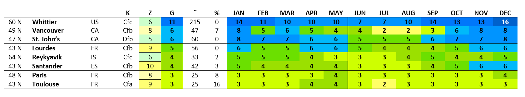
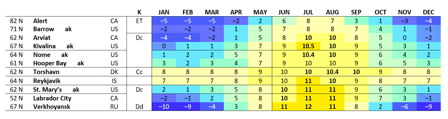
The transitional zone on both sides of the treeline appears to be quite narrow, again, as based on a limited investigation. In any case, to the extent these can be discerned from photos and videos of the locations available through the internet, these discrepancies are indicated by 10+ and 11‒ respectively (in the northern hemisphere). The purpose of this is to avoid as much as possible a potentially glaring misclassification, for example, a summer-zone 11 “temperate rainforest” without trees—zone 11 in such a case being at or near the borderline, for example 10.5, which can be identified as 11‒. Think: “+” = with trees, “‒” = without trees.

In the following chart, months at or above Koppen’s 50^o F threshold are shown in bold. This threshold does not seem to accurately identify the location of the treeline in the northern hemisphere as some of the Dc climates are part of the boreal forest and some are part of the tundra. Kivalina will be identified as 11‒ in accordance with the explanation given above, while Torshavn would be identified as 10+ except that the trees growing there are non-native species from South America, its natural environment appears to be that of a temperate tundra.

Holdridge’s life zones

Koppen’s system, (1918, the first of its modern versions), constituted a major advance in worldwide climate classification; Holdridge’s system, first published in 1947, in certain respects the most significant advance in world bioclimate classification.

Holdridge’s orderly, triangular arrangement of the world’s life zones (biomes, ecosystems) is based on the temperature range within which plants are “active” as opposed to being seasonally or even quite temporarily dormant (annual biotemperature or Bt); annual precipitation totals; and the belief that the life zones are properly delineated, that is, most in agreement with the natural vegetation zones, when these two factors are organized in logarithmic progressions, each range being double the one before it as in a geometric series (for example, 1, 2, 4, 8…).

On the question of precipitation, let’s take for example Mumbai India and Manaus Brazil, two cities with similar annual precipitation totals and falling within Holdridge’s tropical moist forest category—a range of roughly 80 to 160” of average annual precipitation.

A quick comparison of their monthly precipitation totals will suffice in this case because the difference between their precipitation patterns is so obvious, but the grades and aridity percentages will reveal even more. Either way it doesn’t take much to realize that we are dealing with two very different kinds of ecosystems. The dry season in Mumbai is 8 months long, 7 of which qualify as desert-dry. With an aridity index of 58% it is not too far distant from the border of the desert climate; in the grade system it will qualify as a very dry forest. Manaus, in contrast, has a 3-month long dry season and a low aridity index—4%—thus falling in the rainforest grade. A little more research will quickly provide us with at least general support to these determinations: Mumbai is in a “mixed deciduous forest” zone (see for example, Wikipedia: Aary Forest) while Manaus is surrounded by the Amazon rainforest. Clearly when it comes to determining the life zone in question the seasonality of precipitation is decisive.

Having no way to quantify the seasonality of precipitation, Holdridge included its consideration amongst the secondary questions in the subject of bioclimate classification and therefore to be addressed “as needed” and only after the determination of the life zone. When it came right down to it, however, only monsoonal and mediterranean seasonality were actually considered problematic by Holdridge—the result of “abnormal atmospheric conditions”(!) and other things of that caliber—as if the many other patterns of seasonal precipitation either did not exist or were somehow adequately defined by his system. In any case as it turns out, average annual precipitation will be the only definite measurement used in Holdridge’s entire system.

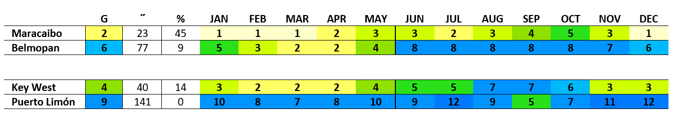
Below we compare climates found in adjacent categories in the Holdridge system according to precipitation, since the transition from one life zone to the next is supposed to mark a step and not a leap. In the first example, Maracaibo Venezuela, a very dry forest, which is next to the dry forest category which includes Belmopan Belize. Here we see they are 4 grades apart; the former is a brushland with a 10 month long dry season, the latter a rainforest with a 3 month long dry season. Both have medium amounts of aridity with respect to their grade and in that sense are “average”.

In the second example, we compare Key West USA, a tropical dry forest which is next to the tropical moist forest zone of Puerto Limón, Costa Rica, a difference of 5 grades. In our system Key West qualifies as a tropical woodland with a lengthy dry season, and Puerto Limón a tropical rainforest, with no dry season at all. (Incidentally, Holdridge’s tropical rainforest starts at around 325”/yr which will exclude almost all of the earth’s tropical rainforests).

And finally a comparison of Belmopan and Key West, both tropical dry forests in Holdridge’s system. Unlike the 80”-wide tropical moist forest range in the example of Mumbai and Manaus given above, this range is about 40” wide, thus leaving much less room for misclassification. Nevertheless, Belmopan is 2 grades wetter, has 37 more inches of rain annually, and has a 4-months-longer rainy season and half the length of the dry season found in Key West. Again, according to their humidity and aridity indexes, the former is a rainforest, the latter a woodland.

Another kind of misclassification results from Holdridge’s recalculation of biotemperature in 1966 which ended up transferring many tropical climates into a supposed “effectively wetter” subtropical zone. This change was not used in characterizing the climates in this section not only because it confuses things further but also because Holdridge-based maps do not always follow this rule. Hence, all of these locations are considered tropical such as they were in the earlier version of his system, not to mention everywhere else minus some differences over thresholds.

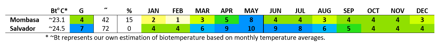
A single example—the case of Mombasa Kenya and Salvador Brazil— should be enough to show what we are talking about here. The fact that these are both considered tropical dry forests in Holdridge’s system is already a big enough stretch in our sensibilities given that their climates are quite dissimilar, Salvador having a rainforest climate with no dry season, and Mombasa, a woodland climate with a 5 month long dry season in total—very nearly a semi-dry woodland climate. Once we introduce Holdridge’s upper limit in the calculation of biotemperature the situation becomes even more untenable because Mombasa, being noticeably hotter than Salvador, will have a biotemperature that is low enough to transfer it into his so-called subtropical zone (26.3 > ~Bt 23.1), whereas Salvador registers hardly any difference between its average annual temperature and biotemperature (25.6 > ~Bt 24.5) and therefore remains in the tropical dry forest life zone. Consequently, we end up with a situation whereby the “dry forest” of Salvador has 30 more inches of rain, is 3 grades wetter and 15% less arid according to its index, has 5 more rainy months, and so forth, than the post-1966 “moist forest” of Mombasa.

In the L & L system no such gross misclassification would ever occur: even if for some reason Mombasa was classified as subtropical, it would remain in the woodland category, and ditto for Salvador in the rainforest category.

Again, the additional oddity that comes with all this is that Mombasa is now classified into a cooler temperature zone which, as we have said, is “effectively wetter”, but only in the sense that the rate of evaporation is lower on average. Yet it is precisely its higher temperatures (hence, lower biotemperature), which necessarily result in a higher rate of evaporation on average and gives the city a “hotter and drier aspect” according to this line of thought, that have caused it to end up in this “effectively wetter” zone. (It has to be wondered why Holdridge’s potential evapotranspiration ratio is still calculated from biotemperature in cases where it has been lowered due to temperatures over 30^o C). In fact, tropical deserts often register the greatest differences between the average annual temperature and corresponding biotemperature, and could therefore very well end up in the even cooler and “wetter” warm temperate range.

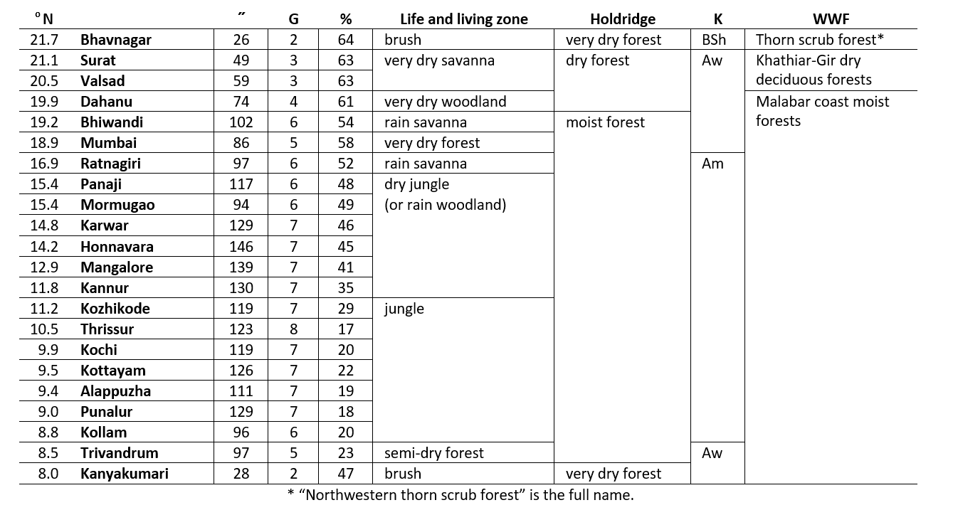
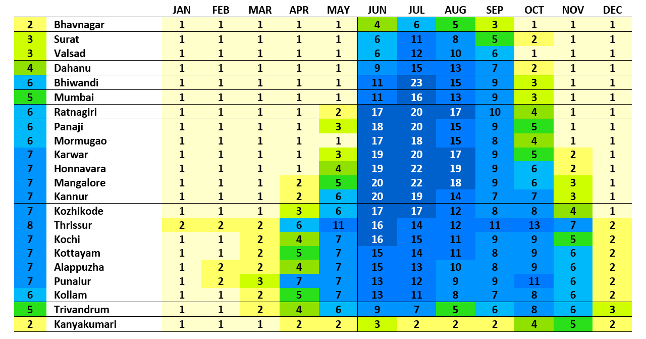
India’s Arabian Sea Coast

The Western Ghats line most of this 1000-mile stretch along the Arabian Sea coast. As shown below, the life and living zones reveal 8 bioclimates—not to be unexpected alongside and within mountainous regions—as opposed to 3 in each of the other descriptions.

As demonstrated above, Holdridge’s logarithmic organization of the life zones according to precipitation creates very obvious problems when two locations have very different seasonality patterns. It can also create problems, however, when the seasonality patterns are closely related, for example, when we compare Thrissur and Mumbai, often considered to have the same bioclimate or share the same ecoregion. Both are part of Holdridge’s tropical moist forest life zone, yet Thrissur is bordering on a rainforest climate, being a half percent (0.52%) beyond its limit. Again, with an aridity percentage of 58.3%, Mumbai is fairly close to the desert bioclimate. The two locations are separated by 37” in annual rainfall, 3 grades, and an aridity index of 42%. Although they are united in the sense that they are both located on the rain-capturing side of the mountains and are drenched by India’s southwest monsoon, the similarity in terms of bioclimates ends there.

Holdridge’s biotemperature zones

Biotemperature (Bt) is Holdridge’s measurement of the temperature range within which, as he put it, “plant growth processes are active”, thus, average annual temperatures above 0^o C, the freezing point and, according to Holdridge’s revised system, up to an estimated 30^o C (32 to 86^o F). A logarithmic progression of biotemperatures delineates the climatic zones—tropical, subtropical, etc.—and thus, together with his logarithmically delineated precipitation zones, the world’s major vegetation zones are supposedly indicated.

We have already seen what happens when we apply a logarithmic progression to annual precipitation. In the case of biotemperature one of the first things we discover is that half of his zones—Bt 6 through 30^oC—are not even in logarithmic progression but form an arithmetic series based on the multiple 6—Bt 1.5, 3, 6, 12—18—24, 30^oC. Equally perplexing, his tropical range beginning at Bt 24^oC should in theory extend to Bt 48^oC, whereas on his chart it is cut off at Bt 36^oC.—But even this is not quite so: Holdridge informs us that the warmest climates on earth “scarcely exceed (Bt) 27^oC”. In short, a rough 7/8 of Holdridge’s tropical range is empty, a feature of his system which has no apparent justification. If we calculate biotemperature using an upper limit at Bt 30^oC as did Holdridge in the final version of his system, the actual tropical range, although not necessarily narrower, will lose many of its locations to the subtropical range. As we begin to examine actual climates in their different ranges we will discover that—much as was the case with the precipitation series—the results of the use of the biotemperature series will range from more or less passable on its lower, narrower end, to entirely dubious on its higher, wider end.

Discovering the lessons of biotemperature in either Holdridge’s Life Zone Ecology or from his diagram of life zones is not going to be easy. The fact alone that his precipitation and temperature ranges are organized in two very different manners is already an indication that Holdridge seems to have been quite perplexed by it all, by biotemperatures, the logarithmic progression, and so forth. A comparison of climates according to biotemperature would be enough to demonstrate that Holdridge’s system is not creating zones of “equal weight”, but this is so much easier said than done: Holdridge leaves the “average investigator” of his system with a single tool—a “rough” calculation of biotemperature based on average monthly temperatures—only valid in the “colder regions, towards the poles”. His single example, Verkhoyansk Russia, is one of the coldest cities on the planet and leaves the reader to wonder where the “colder-region climate” begins and ends. Given the tremendous importance of biotemperature to his theory and system, and the fact that its calculation is necessary in order to start testing and making practical use of his system, the whole thing is completely odd. At this point our “average investigator” is pretty much left to either accept the system and any Holdridge-based maps out there on good faith or walk away from the whole thing empty-handed.

In order to understand biotemperature, the first thing we are going to do is “correct” Holdridge’s series in the simplest manner possible: Bt 1, 4, 9, 16, 25, 36^o C, which is an arithmetic series of square numbers using Celsius. This is by the way the first time we use Celsius instead of Fahrenheit, the latter together with the imperial system (inches, feet) having thus far served as the “language” of climate classification. Celsius works so well here because biotemperature ends at the point that water freezes and plant activity more or less comes to a halt, hence, fittingly, “point zero” or 0^o C.

Next, we are going to turn this series into temperature grades (tg)—1, 2, 3, 4, 5, 6—a format similar to that of the precipitation grades (pg), although not nearly as extended. Whether we use biotemperature of convert the series into grades, what we have is an effective warmth index or the average annual sum total of “warmth”—temperatures above freezing—in any given location. This in itself is a useful figure when comparing climates in their own right, that is, without any particular reference to the ecosystem and plant biology. Additionally, the warmth index provides us with an excellent overall view of the climate, except that it tells us nothing specific about “winter”, that is, in the sense of monthly temperatures below freezing. In the final analysis, both climate and bioclimate classification require both measurements.

The rest is a matter of testing the “corrected” series in order to determine its demarcation points more precisely. Two things were taken into consideration in doing so:

1) The tropical range should be full or at least very nearly so. If the whole numbers of the new series are used as the points of demarcation, the tropical category will still be half empty as it ends around 5.5 or midway between 5.0 and 6.0. Although this is a major improvement when compared with Holdridge’s model, it is neither desirable nor even accurate as many “plainly tropical” climates are found below 5.0; and, well if the reader wants to see what a 6.0 climate looks like, google Dallol Ethiopia, images, keeping in mind that this former mining town is over 400’ below sea level, hence need not be considered any further at the moment.

2) The climates at the extreme ends of any particular range, as opposite as they may appear from each other, still have to be seen as relatable. Setting the limit of the tropical range to Bt 30.5^oC to accommodate the hottest climates so far found (at or above sea level) we derive the multiple 0.9204 and the series, rounded to the tenth:

0.9, 1.8, 2.8, 3.7, 4.6, 5.5

The first grade, 0.92, is frigid; the second, polar; the third, subpolar, and so forth. A “simplifying multiple”—1.086429—could be introduced at this point so that the frigid grade ends at 1.0; the polar grade at 2.0…the tropical grade at 6.0. For example, 4.5 x 1.086 = 4.88 or rounded up to the higher whole number, grade 5 = subtropical, and named as such if the zone is also subtropical. If the zone is tropical, however, the climate is called ‒tropical. Nothing of course prevents us from identifying a sixth-grade climate (4.6 to 5.5) as such, that is, without introducing the “simplifying multiple”. In any case, such a modified system may be introduced in the future if people find it more appealing for whatever reason.

The multiple 0.92 can be tested anywhere within the system, not just at the demarcation points. Starting from the tropical grade, nevertheless, Bakel Senegal at 5.5 and Las Palmas Spain (Canary Islands) at 4.6 represent its extreme opposite ends. An alteration of the series-defining multiple could knock one or the other of these locations out of the category, opening up the subject to an endless debate over what is essentially a minor difference.

Only dry climates have been found in 5.5 so far whereas in 5.4 we begin to find some wet climates. Towards the opposite end of the tropical category we are already finding tropical climates that have been substantially cooled down by the effects of altitude, cold offshore currents and whatnot, or, conversely, have been substantially heated up by warm ocean currents in spite of their location well beyond the tropical latitudes, at 32^oN and grade 4.7 Bermuda being the best example. The climates found below 4.6 are called “‒tropical” and are a continuation of these types; they are generally characterized by their year-round, sometimes more, sometimes less-than-comfortable spring-like weather.

Meanwhile back in Holdridgeville, noticeably hotter places like Rio de Janeiro and even hotter San Juan Puerto Rico, the latter if we calculate with the upper limit of biotemperature, are still classified as subtropical; here of course at tg 4.9 and 5.2 respectively these are near the middle of the tropical grade. This is surely another one of those very strange items we find when examining Holdridge’s system: “subtropical” climates that appear completely tropical.

A similar ambiguity between what is tropical and what is subtropical seems to be common in the subject of ecoregion classification as well, whereby for some reason not yet discovered—but perhaps taking lessons from Holdridge—the two climates and their ecosystems are often-times classified together. However, as we are about to detail below, the overlapping of zone and grade occurs throughout the system and is actually increasing as the climate gets colder and colder. In this regard then, the tropical grade is more “compact” and consequently more distinct than all the others as it comprised of only 6 zones—4 tropical and 2 subtropical—and is therefore the least suitable for any sort of broader combination.

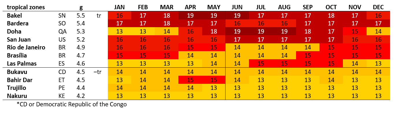
To be clear, once the temperature grade becomes part of a climate’s description, not every climate according to its zone is hotter than a climate according to its grade. Kuwait City, for example, is considered +subtropical or subtropical by zone and tropical by grade. Thus, once its seasonality is taken into consideration it is notably warmer than many tropical locations—Miami (5.0); Honolulu and Santo Domingo (5.1), to name but a few. Only Kuwait City’s subtropical-zone winter excludes it from the tropical category.

The cooler subtropical climates (especially those in ‒st) resemble oceanic climates, except that, apart from Dinard and La Rochelle France, their precipitation pattern doesn’t qualify them as such. At the other end of the spectrum, many of the warmer subtropical climates (+st) have a somewhat opposite character in that these consists of deserts or climates with long dry seasons.

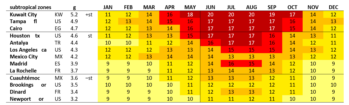
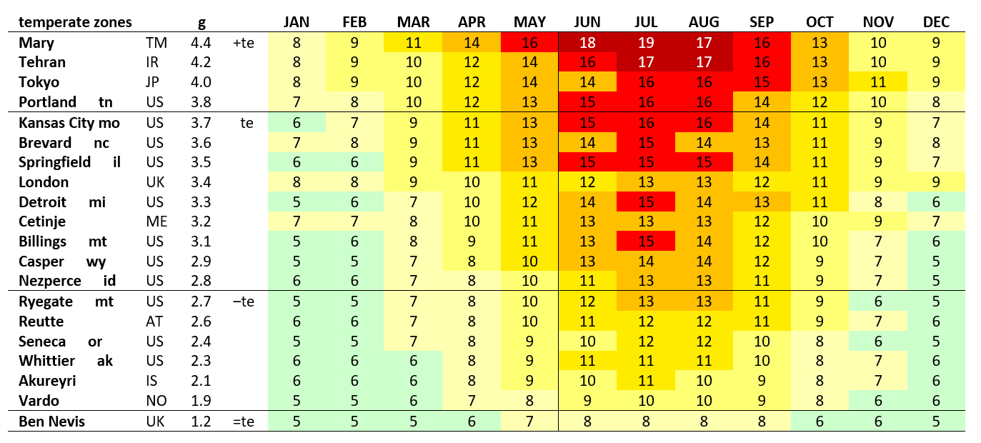
Again, owing to the difference between a calculation based on the coldest month of the year and the measurement of seasonality based on “warmth”, the gap between the zones and grades as indicated by their names increases as we progress from the tropical to the polar climates. By the time we get to the subpolar zones shown below, we find nearly as many +subpolar grades (by tenths) as we do subpolar climates. Minus the fact that their winters dip into the subpolar zones, these climates appear more temperate than subpolar. Nevertheless, it should be noted that their seasonal differences are more marked than those found in the fully temperate category since in order to be “+subpolar” their colder winter has to be offset by a warmer summer. In short, we have some pronounced examples of the continental effect in climatology, somewhat comparable to the concept of Koppen’s “humid continental” climate, although not necessarily humid nor so loosely defined. In the chart below only Bedford and Dubuque Iowa qualify as humid (grade 4, semi-wet), while the remainder are located in the dry precipitation grades (1, 2, and 3).

Continental effects result from the rapid heating and cooling of the land mass over the course of the year and are thus typical of the continental interiors, that is, away from the moderating effects of the ocean which heat up and cool off much more slowly. In North America the continental effects are much more pronounced than in northern Europe because the oceanic effects are largely contained by the Rocky Mountains. At the same time, however, this means that the “humid continental” climates on the eastern side of the Rockies are necessarily going to be quite dry, that is, until we reach the eastern states as these receive additional moisture from the Gulf of Mexico and in some cases, especially along the seaboard, the Atlantic Ocean. If we go far enough north along the seaboard, the “humid continental” climates are once again oceanic, albeit somewhat colder versions, for example, St. John’s Canada.

Notice that the subpolar climates range from 1.8 to 2.8: this is only because the grades have been rounded to the tenth at which point the borderline climates are determined by the name of the zone, here and throughout the system. This little bit of “wiggle-room” built into the system helped to reduce the use of the + and ‒ signs somewhat. On a somewhat negative note, however, it means that the names of the system will not reversible in borderline situations. Put another way, without allowing for some wiggle-room, a “‒tropical climate” by zone can also and always be considered a “+subtropical climate” by grade. Practically speaking, it won’t really matter since any climate identified primarily by its grade for whatever reason, still has to be distinguished as such, otherwise the names become ambiguous.

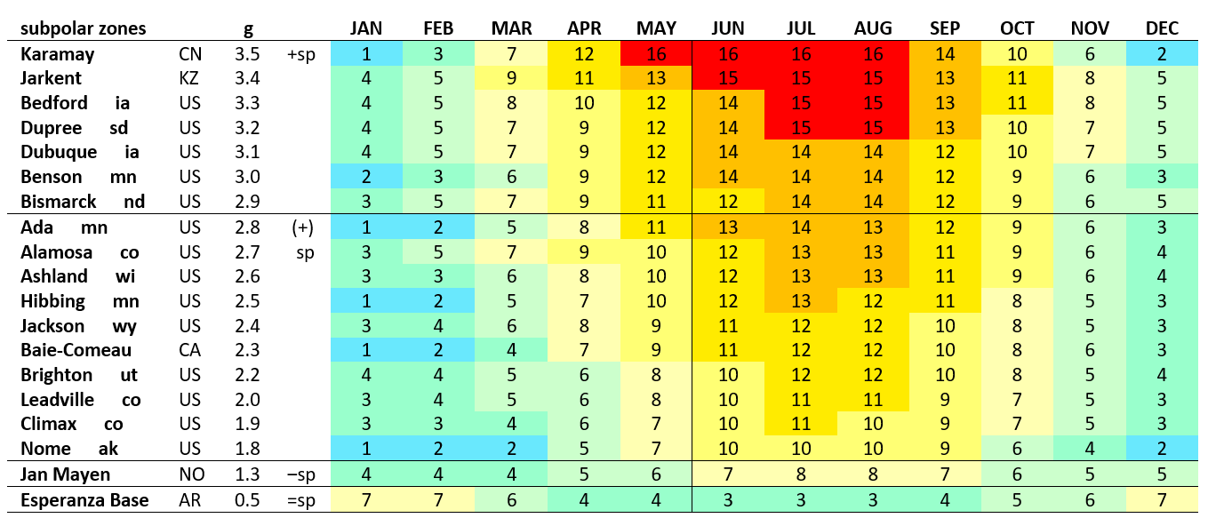
As we progress into the polar regions we find more of the same, that is, polar-zone climates that are more subpolar than polar.

Grade 5.5—Bt 30^oC—is the approximate limit of the tropical range in terms of average annual temperatures at sea level. Seasonal temperatures can be significantly higher, however. For example, Ahvaz Iran has a tg of 6.0—Bt 36.0^oC—in summer, peaking at 6.1—Bt 37.3^oC—in July. Death Valley, which is below sea level, has a tg of 6.2 in summer and 6.3 in July.

Bt 30^oC (86^oF), or something close to it, happens to be identical to Holdridge’s upper limit of biotemperature introduced into his system in 1966. Accordingly, above this temperature, plants supposedly shut down until temperatures go back below this temperature. Even today, this figure is still regarded a kind of general upper limit of the range within which plants grow best. Above that, the heat—especially intense and prolonged heat—starts to seriously affect the health of the plant. Clearly, although Holdridge’s system is supposed to describe the natural vegetation, his upper limit of biotemperature is really only applicable in agriculture and horticulture, that is, where plants, now often found outside of their native climate, are cultivated to whatever ends and the propagation of the species is largely or entirely dependent on human intervention.

The “goal” of plants in their natural habitat ultimately comes down to their reproduction, hence, the “upper limit” is species-dependent. However, since species evolve within a given range of temperatures to begin with, heat stress to that point where the reproduction of the species is seriously threatened can only really occur quite beyond that range. In Ahvaz, for example, the average high in the month of July is 47^oC (116.6^o F) and the average low—still above the 30^oC threshold by the way—is 30.5^oC  (86.9^o F).  In spite of these extreme temperatures, we still find ample vegetation alongside the Karun river in what is otherwise a desert. Assuming that this vegetation—although possibly introduced by humans—is reproducing itself without human intervention, the mean maximum temperature for July—53^oC (125.6^oF)—would establish at least a “local” and average upper limit of biotemperature, that is, one that is valid for the species found in that region. Propagation-threatening temperatures would have to be higher still and probably of some duration. Long story short, all of these figures are quite beyond Holdridge’s upper limit. Pending verification, Death Valley also supports some vegetation beyond the saltpan and according to water availability in any given year.

Uncertainty surrounds just about everything having to do with biotemperature as discussed by Holdridge: its benefits or precise significance, its limits, its calculation, its organization in logarithmic progression, and not the least of it, Holdridge’s peculiar obsession with frost, that is, 0^o C (32^o F), the point at which water freezes and the lower limit of his biotemperature. Ultimately, the validity of his logarithmic series is not proven, not to mention it has also been compromised and corrupted by his frost line, and later further confused by the introduction of the upper limit of biotemperature.

What happens when we increase biotemperature? When we increase biotemperature we find that the diversity and productive capacity of the plant life increases, although in accordance with the availability of water. According to precipitation alone, the effects of biotemperature will be offset by the precipitation grade and aridity index, for example, a very high biotemperature and very low precipitation grade will result in a tropical desert and aspect assuming no other source of water.

On the fringes of the frigid desert where biotemperatures are at their very lowest, when we do find vegetation it does not necessarily appear every summer being dependent on a sufficient summer thaw which can vary somewhat from one year to the next. As biotemperature increases we see the regular formation of the tundra in the short chilly summer. Up to this point the amount of precipitation does not fundamentally alter the overall appearance of the desert or tundra, or for the matter, according to the temperature grades, any of the forested locations falling within the polar brushland range (tg 0.9 to 1.8, that is, the main range of the tundra).

Following the tundra in Holdridge’s system, beginning at around 10” in annual precipitation, we have the boreal forest, following that, the temperate forest, and so forth. At this point on Holdridge’s chart of life zones, however, given an equal amount of precipitation, the aspect of the environment starts to decrease with the increase of biotemperatures—hence also an increase in the rate of evaporation—such that, in the down-to-the-left direction on his chart ( ↙ ), the boreal rainforest, is followed by the cool temperate wet forest, the warm temperate/subtropical moist forest, and the tropical dry forest. This is a very particular assumption, but from what has already been said about the organization of Holdridge’s system we can say with absolute certainty that this is not going to produce consistent results: The “tropical dry forest” climate of Salvador Brazil, part of the Atlantic Forest ecoregion, exhibits a level of biodiversity comparable to that of the Amazon rainforest which is very high. Holdridge’s “boreal rainforest” on the other hand—Highmarket New York, for example—cannot possibly match, let alone surpass this level as it is limited from the start by its much lower temperature grade: 2.7 as opposed to 5.1 for Salvador.

Grades are direct indicators of biodiversity and productivity, 0.9 = little or no biodiversity and productivity at all; 1.8 = very low; 2.7 = low and so forth. Parallels can be gathered from the animal kingdom since a part of it is dependent on the vegetation for food to one extent or another and the other part on the herbivores likewise.

Perhaps biodiversity will be more readily understood when precipitation totals are doubled from one range to the next such as we find in the remaining 2 directions across Holdridge’s triangle. Viewed horizontally, this will effect a change of life zone when using the same biotemperature (or range of biotemperatures), for example, cool temperate steppe (10 to 20”) → cool temperate moist forest (20 to 40”), etc. Considered in the other direction ( ↘ ) the “constancy” or aspect of the life zone—a “moist forest”, for example—will be maintained while the biotemperature increases: boreal moist forest (10 to 20”) ↘ cool temperate moist forest (20 to 40”).

In terms of consistency and accuracy of the results, these formulations can be no more precise than the formulation given above whereby the amount of precipitation remains the same while the biotemperature increases. It is simply not possible that the system, being interconnected in the triangular format as it is, can function accurately, let alone be properly named, in one direction but not the other two. More fundamentally, however, the triangular format and system of names gives the impression that any evapotranspiration is simply “water lost” rather than referencing the fact that part of the “lost” precipitation has already been used and even stored away for future use in some species. There is certainly more to consider when it comes to evapotranspiration, mainly, however, whatever significance it has appears to be greatly exaggerated by the triangular format whereby increasing biotemperature, hence evapotranspiration, results in a “downgrading” of the environment given an equal amount of precipitation, for example, subtropical dry forest ↙ tropical very dry forest. Even more generally speaking, the consideration of evapotranspiration seems to assume a much greater role in bioclimate classification owing to the lack of a concise calculation of seasonal precipitation, which is of course something we now have in the precipitation grade and aridity index.

In  the L & L system, in order to effect a meaningful change of life zone by doubling precipitation totals, the “time factor” or number of precipitation days have to be doubled too, hence, both measurements forming a logarithmic progression. The precipitation grades and derivative aridity index are then displayed into a convenient rectangular chart representing the year divided in such a way as to indicate degrees of seasonality (a percentage of the year).

√(days x inches ÷ 365) = precipitation grade or index (annual)

Having been the creator of biotemperature Holdridge could have eventually uncovered its benefits but rather than bring the viability of his system into question and re-examine his methodology, Holdridge insisted on patching his system every time a problem came up which of course only made the contradictions worse. The fact of the matter is that as long as biotemperature remained trapped in his logarithmic, triangular format with all of its entanglements, it too becomes “suspect”, adding to the uncertainty of it all. Besides this, even a basic classification model requires a description according to zones as well. The closest we get to this is Holdridge’s frost line, a single marker at or around Bt 18^oC that is otherwise so absolute it is no longer realistic in spite of the “critical” significance attributed to it by Holdridge and the adherents of his system.

Although Holdridge’s instructions are characteristically not explicit, in climates where the mean daily maximum is at or below 30^o C, including all of the locations listed in the chart to follow, a “rough” biotemperature can be determined by adding together the monthly temperature averages above 0^o C and dividing the result by 12. The answer will determine the range within which the climate in question will be located, for example, Nome Alaska with a biotemperature of 3.28^oC falls within his tundra life zone (Bt 1.25 to 3.5^oC) which is about equal to our polar = very low biodiversity range (Bt 0.9 to 3.3^oC). Even if trees began to take hold around Nome—it wouldn’t take much for this to happen in terms of summer temperatures—it might require a little more than that to transfer Nome into the next range of biodiversity (Bt 3.3 to 7.5^o C). And again, if a forested Nome were to fall in this higher range, the amount of precipitation would more and more have an effect on the overall appearance of its environment: for example, more trees, taller trees, more species, etc., or a combination of these and/or other descriptions according to the species present and their adaptations to the environment.

Before moving on, it should be pointed out that the Holdridge’s “rough calculation” of biotemperature is as legitimate as any other daily mean considered month by month. In all such cases the general picture is satisfied while some of the particulars, requiring day by day averages, are smoothed over in the month-by-month format.

The following chart, representing half of Holdridge’s ranges, shows us that the major ecosystems are not always well-defined by the ranges even though these ranges are on the narrower half of the chart where there is less room for error—and the life zones bear their names. The tundra (Bt 1.25 to 3.5^o C), most of which falls in his subpolar category (Bt 1.5 to 3^o C), seems to be an exception to this rule at first except for the fact that, having such a narrow range, it really only includes a portion of the tundra while the rest of it is found in categories identified by other ecosystems. We also indicate the temperature zone of the warmest month of the year which is a necessary indicator of the tundra, the dotted line below representing the treeline, excluding locations in South America.

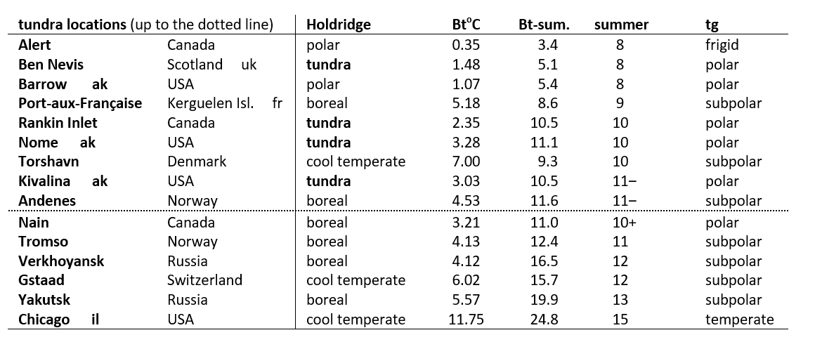
At this point, a few more examples and some background information should be enough to demonstrate the utter uselessness of Holdridge’s system. The reader may recall the example of Kansas City and Tampa described earlier, two locations which cannot possibly be considered as similar in terms of temperature or vegetation, but nevertheless belonging to Koppen’s humid subtropical category. While Koppen’s category spans 7 of our temperature zones—zones 6 through 12—Holdridge’s equivalent category—after splitting the Warm Temperate range in two of course—is still at least two zones wider—5 through 13—and is still dipping into the tropical climate zone. Additionally, as shown below, tropical climates by most every other standard are regularly distributed amongst 3 different categories in the Holdridge system, many of the “subtropical” climates being indistinguishable from the tropical. Nevertheless, in this otherwise mind-boggling arrangement of climates which we will attempt to get to the bottom of soon enough, we will manage to salvage one single element lurking within it—the frost line—oddly enough the same element that spells the end of his system. Until that time, however, the system of temperature zones defines St. Joseph Missouri as temperate, Tampa Florida and Marsala Italy subtropical, and the rest tropical.

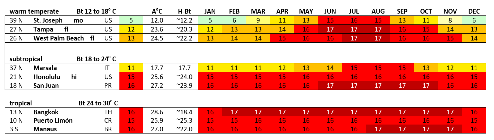
The really defective nature of his system seems to have fully stood out for the first time when Sawyer, while mapping out Florida’s life zones, discovered that those climates having a subtropical biotemperature fell on the wrong side of Holdridge’s “critical temperature” or “frost line.” At least in the case of Florida, Holdridge’s subtropical zone was completely empty. Obviously a life zone map of Florida with a blank spot on it would not do, so in his response to Sawyer the otherwise frost-sensitive Holdridge suggested replacing frost (0^o C) with a “killing frost” set at ‒2^o C: if this occurred less than once every 3 years on average, the location could still be considered subtropical; more than that it would have to be considered warm temperate in spite of its biotemperature. Thus, Sawyer—thanks to the new uncritical temperature or killing-frost line—was able to insert a small subtropical zone in central Florida between the vast warm temperate and tropical zones around it. The Sawyer map was now presentable (as opposed to not even possible before), but could hardly be considered satisfactory: again, the subtropical zone was very small in spite of Holdridge’s manipulations, and, of course, it still didn’t add up since the warm temperate zone now had climates with the wrong biotemperature in it. It was more than beginning to look like Holdridge’s system was not merely “defective”, but actually beyond repair.

Not long after the publication of Sawyer’s work, while Holdridge was on a mapping expedition on the island of Hispaniola in the West Indies, he made an observation regarding the local vegetation that was going to have definite consequences with regard to his system of life zones… There, according to Holdridge:

It was noticed that the vegetation at low elevations on the island had the appearance of that of higher elevational vegetation in the inner tropics. (…) Since the low elevation vegetation in the outer tropics appeared to correspond more closely to that at somewhat higher elevations in the inner tropics, the obvious conclusion was that there must be some maximum temperature cut-off above which vegetative growth becomes insignificant. (Life Zone Ecology).

And pretty much just like that Holdridge established an approximate upper limit in the calculation of biotemperature at 30^o C (86^o F), above which, at least for some or perhaps many species, vegetative growth is temporarily suspended until temperatures go back below 30^o C, and that all of this is somehow of great significance to basic bioclimate classification. This is classic Holdridge: introducing items into his system which will vary according to the species, in this case some species being able to tolerate or even require periods of high heat—or whatever conditions are part of the environment in which they have evolved or have become naturalized. For example, his “killing frost”, which as is well known and he himself acknowledges, varies widely between species. Still again, his potential evapotranspiration ratio which is also dependent on other factors, including climatic ones such as wind and sunshine duration, etc., moreover a figure which even Holdridge declares “not amenable to measurement”. As for the natural vegetation meanwhile, it is already “adjusted” to whatever amount of moisture may be lost to evaporation, absorbing what they can, when they can, in order to thrive and reproduce. Yet Holdridge places these “variables” or species-dependent considerations—which by the way are mainly considerations of agriculture—(and it’s not like we’re going to take measures like watering the natural vegetation when evapotranspiration is high, etc.)—he places these things in the worst possible location, that is, in the foundation of the system itself.

Holdridge presented his “discovery” of biotemperature’s upper limit as an “unfortunate complication in the calculation of biotemperature”. It could, however, be seen as an incredible stroke of luck…maybe even too incredible: Suddenly, having found a reason and a way to lower their biotemperature, Miami, Hispaniola, and many a tropical location and getaway were swept into the subtropical zone, actually constituting its main variety. Holdridge even provided the subtropical zone a large territory of its own, asserting that it continued as far south as the 13^th parallel, thus forming the “outer tropics”—at least in the northern, western hemisphere.

All of this rest on a whole series of assertions actually, the immediate one, however, being that as a general rule the outer tropical lowlands resemble the inner tropical highlands on account of similar biotemperatures. The most obvious problem with this proposition is that the highlands have lower biotemperatures—often approximating or equal to their average annual temperature—simply because they are cooler, whereas the hotter lowlands have lowered biotemperatures because they are extremely likely to go over Holdridge’s 30^oC threshold for some period during the year if not throughout the year. Assuming an equal amount of annual precipitation, how is it possible that a cooler and “effectively wetter” environment (that is, in terms of a lower rate of evaporation) resembles a hotter and “effectively drier” location?

Without a convenient formula to estimate the upper limit of biotemperature from monthly temperature averages, the negative effect of this change on his system tends to get lost in the confusion. According to Holdridge a “reasonably accurate” biotemperature requires hourly temperatures readings for the entire year, presumably the standard 30-year period providing us with an accurate biotemperature. Once again, for the average investigator of his system there is almost no getting beyond the first step—the calculation of an accurate biotemperature. (There are actually a few ways to get around this problem using monthly temperature averages, simply Holdridge doesn’t know or doesn’t tell his readers what these are).

In any case, all of these things help to explain the bizarre results shown in the examples above. Naturally, other results are also possible because Holdridge explanations are bare minimalist if not openly contradictory, or are simply absent. How did such a situation ever come about in the first place?

In many respects it seems to boil down to the frost line—that first really obvious sign of trouble Sawyer had when mapping out Florida’s life zones: it so oddly cuts right across a range of life zones, splitting it into two groups, and yet it does not separate the subtropical climates from tropical climates as we should expect, but the frost-having temperate climates from the frost-free subtropical climates. So first off, before the introduction of the upper limit of biotemperature, when we speak of a frost-free climate in terms of Holdridge’s system we are speaking of a climate where biotemperature and temperature have merged into a single figure. The point at which this merging begins is indicated on his life zone chart by the frost line at 18^o C although Holdridge said it probably varied between Bt 16^o and 18^o C. But why insert a frost line at all?, and why such an “absolute” frost line? At 18^o C it basically resembles Koppen’s demarcation of the tropical climates which, however, is based on the average temperature of the coldest month of the year. While Koppen’s de facto frost line is not so absolute, it is much more practical and consistent with the “big picture”.

It must have all started while Holdridge was in the tinkering stage of his project, that is, organizing his biotemperatures in logarithmic order into a meaningful and harmonious chart. Unfortunately, due to the constant doubling of ranges, the best possible arrangement he could come up with rendered his undivided Warm Temperate range (Bt 12 to 24^oC) completely unrealistic. In short, the logarithmic progression had outpaced the progression of climates, thus causing two very different climates, for example, St. Joseph Missouri and Rio de Janeiro—a range of 10 zones—to end up in the same category. Divided, half of his system consists of equally sized ranges (6^o C each), thus no longer forming a logarithmic progression. There are no reasonable solutions here. In fact, ultimately, his division of the Warm Temperate range only meant that the zone 14 climates below an average annual temperature (also the Bt) of 24^o C—Rio de Janeiro in the example above—would now be called subtropical, rather than Warm Temperate. It may have sounded more reasonable but the underlying problem remained unsolved.

We know of course that Holdridge opted to split the Warm Temperate range as that is how it has always figured since his system was first published in 1947. But a divided range upsetting the harmony of his system?—that was definitely going to require some sort of justification. Therefore, he had to insist that the subtropical climates be completely frost-free. After elevating the status of the frost line to the “critical temperature line”, the only thing left for Holdridge to do at this point was to blame it all on Nature—not on his system—by declaring frost to be “the one great anomaly in the progression of life zones.” He couldn’t possibly have been more mistaken—and not only from the standpoint of the temperature zones and the biotemperature series (corrected), both zone 12.5 and Bt 0.9^oC “setting the pace” of the series to follow, but also from the standpoint of his own system as there is no need for biotemperature without the presence of frost and its effect on plant biology and the species present.

After the Florida-mapping fiasco, desperate for a more attractive solution or probably, at that point, just a better-looking map, Holdridge eventually decided to fill the subtropical zone with tropical climates by lowering their biotemperature on the basis that some of these are too hot (!), that is, by giving biotemperature an upper limit.

This action only made the contradictions worse than they already were since the hotter the climate the further it advanced towards and into the cooler biotemperature ranges, etc. Not only that, if we follow the new standard consistently, his tropical zone would have to be significantly reduced not only in terms of its geographic territory but also in terms of temperature zones, perhaps consisting of just 3 zones at this point as opposed to 6 or 7—hence, mostly relatively milder tropical climates within zones 15 and 16 which are really not all that typical. This reduction is not always visible on Holdridge-based maps as the mapmakers can always follow Holdridge’s “inner tropics rule” which basically takes biotemperature out of the equation, that is, the idea that the “inner tropics” range from the equator to 13^o N at least in North America.

Oddly enough, with many or even the majority of tropical climates relocated into the subtropical category, the frost line which seemed to serve no other purpose than to make his logarithmic system seem a little more reasonable, actually began to look like a frost line for the first time—not as the separation of frost-having warm temperate and frost-free subtropical climates but actual subtropical and tropical climates. Still though, to be clear, Holdridge never cleared out the frost-free subtropical climates, leaving the new contradictions (samples of which are shown above) that necessarily arose from his actions exactly where we see them today. From start to finish, therefore, we have been largely caught up in a time-consuming exercise in futility, his explanations, methodology, and each and every one of his “fixes” making the system even more confusing and impossible. Very much to his credit, nevertheless, Holdridge uncovered a link between the logarithmic progression and precipitation and temperature averages, between biotemperature and its organization into qualitative classes, and seems to have been the one who introduced the concept the frost line, even though in order to make sense of and actually use these items, each had to be re-defined and rescued from their creator and his mystical-like presentation and triangle.

Together with the precipitation grades and aridity index we have a general description of the vegetation zones, which are zones of biodiversity and productivity based on “warmth” and the calculation of aridity. Other seasonality figures are possible, for example, an upper limit or upper limits of biotemperature according to their effect on agriculture, gardening, with respect to individual species, and so forth, a percentage of the year above a given temperature providing the exact same information; or practical average dates such as the first and last frosts of the year; for precipitation, onset of the rainy season, and so forth.

This concludes our presentation for the time being. We have hopefully left our readers with a clear picture and understanding of the earth’s climates especially as they relate to everyday life and the natural environment itself, these considerations constituting the “best and most interesting parts” of our own system. Our journey having led us to this point, perhaps it is not by chance that the descriptions of climates presented herein can also be seen as a call upon ourselves to restore and watch over the magnificent harmony of life.